This is a project made for EE 475: Introduction to Image Processing course in Boğaziçi University EE Department.
Image stitching is the operation of combining photos taken from the same panorama. This can be done by using the classical approach or the parameters from a convolutional neural network. The classical approach consists of 4 main steps:
1- Detecting Keypoints
2- Matching Keypoints
3- Computing the Homography Matrix
4- Warping and Blending the Images
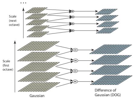
The first step of image stitching is detecting the keypoints/features. This is usually done by using the SIFT (scale-invariant feature transformation) algorithm. SIFT algorithm uses the Gaussian blurred versions of the image and difference of Gaussians (DoG) technique to highlight the keypoints.
Gaussian blur is the operation of blurring an image by using the Gaussian distribution as the kernel of filter. As the sigma value (standard deviation) gets higher the Gaussian function gets more spread out further blurring the image. The strong features on the image get less effected by this filter. Difference of Gaussians (DoG) is a technique for feature enhancement where the Gaussian blurred versions of the image are subtracted from each other.
In SIFT algorithm, first a Gaussian pyramid is formed which consists of Gaussian blurred versions of the image with different sigma values. Then the adjacent blurred images are subtracted from each other creating a DoG pyramid. The lower layers of the pyramid correspond to a subtraction between small sigma values and the higher layers correspond to a subtraction between large sigma values. The keypoint candidates are then found by finding the local extrema inside a 3x3x3 grid on the DoG pyramid. Some of these candidates are eliminated by using a threshold and the resulting pixels are the keypoints. An extrema on a higher DoG layer will be a stronger feature therefore it will be a bigger blob and have a higher magnitude compared to the local extrema on the lower layers.
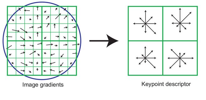
Orientation of the keypoints are then found by finding the gradients accross a grid inside the blog. The most recurrent direction inside the grid is the dominant gradient direction of the keypoint. Finally, scales and orientations of the keypoints are set to a constant value so that the points become scale-invariant which will be pretty helpful in comparing and matching the images.
The keypoints are matched by using a principle called keypoint descriptors. Each detected keypoint has its own descriptor based on its gradient accross the grid inside the blob. To find the descriptor, first the blob is divided into 4 quadrants. Then a histogram of the gradient directions are created for each of the quadrants. This histogram is the keypoint descriptor. Keypoints are matched by looking at the histogram distance between two keypoint. There are a variety of metrics to measure the distance between the keypoints such as L2 distance, intersection, Bhattacharyya distance, correlation etc. To make the calculations easier L2 distance was used in this project.
Sometimes one of the images will have a very distinct keypoint. As a result of that the match of this keypoint will have a very high distance and most probably this will be a wrong match. In order to prevent this we added a distance threshold that only considers the matches under a certain distance value. This correct most of the false matches. The default value is 200 but the user can change this as a command line argument. In addition to that there is also a keypoint threshold. If the number of valid keypoint matches are lower than this threshold the stitching operation will be cancelled. This prevents the creation of wrong homography matrices and therefore wrong stitches.
Now that the keypoints are found and matched, the planes in which the 2D images are located must be transformed to the same plane. This will enable us to stitch the images. Otherwise the image will seem distorted because of the plane differences. This operation is done by finding the homography matrix between the images. This matrix transforms the plane of one image to the plane of the other image. So in other words, the homography matrix transforms the keypoints in the source image to the keypoints in the destination image with minimum error.

Since this matrix has 8 degrees of freedom a minimum number of 4 matches (8 keypoints in total) are enough to find the homography matrix. If the matches are correct it becomes a constrained least squares problem which can be solved by some knowledge in linear algebra. However there are far more matches and sometimes some of these matches turn out to be false. In order to tackle this problem an algortithm called RANSAC (Random Sample Consensus) is implemented. Basically, this algorithm separates the outliers (wrong matches) from the inliers (correct matches).
The first step of RANSAC is to choose 4 random pairs on the images and finding the homogprahy matrix with them. Then this matrix is applied to the other points in order to transform them to the destination image. If the distance between the transformed keypoint and the destination keypoint is lower than some treshold, it is counted as a score. The process is repeated until all the combinations are achieved. Finally the 4 points that have the highest score will be selected as the basis for calculating the homography matrix. This algorithm works pretty well as long as the number of correct matches are higher than the wrong matches. However, one disadvantage is that it takes relatively long to run because all the combinations are considered during the operation.
The final part of image stitching is warping and blending these two images. Warping is the operation of transforming one image to the other one by using the homogrpahy matrix. In the end of this operation images will be on the same plane and ready to be stitched. However, sometimes there are exposure differences between the images. These may cause unnatural brightness differences on the region of intersection of the images. This problem can be solved by applying blending. Even though this step is optional, in some cases it will reduce this unnatural look. Blending is basically multiplying the pixel values located on the region of intersection with a weight and adding them. Since the weights are diminishing towards the edges of the image, the result will seem smoother than the original.
Batu ALPAN
Deniz Altay AVCI